Modelización de la volatilidad y Valor en Riesgo (VaR) del Bitcoin
## [1] "BTC-USD"Contenido
Descripción
1. Especificación de los modelos Garch
1.1 Modelos eGarch
1.2 Modelos gjrGarch
1.3 Modelos TGarch
2. Supocisiones de distribución de error
2.1 Distribución normal
2.2 Distribución T-Student
2.3 Distribución de errores generalizados
3. Criterio de Akaike
4. Preparación de datos
5. Revisión de parámetros del modelo
6. Prueba Ljung Box
7. Prueba de Lagrange Efecto Arch
8. Valor en Riesgo VaR
9. Análisis de residuos
10. Pronósticos
Descripción
Este entrenamiento evaluó la volatilidad y el Valor en Riesgo (VaR) de los retornos diarios de Bitcoins mediante la realización de un estudio comparativo en el desempeño de los pronósticos de los modelos GARCH simétricos y asimétricos basados en tres distribuciones de error durante el período enero-2014 a enero-2020.
Los modelos empleados son el SGARCH, TGARCH, eGARCH Y el gjrGARCH que fueron validados en base a indicadores de la precisión de la previsión: AIC, MAE y MSE. Los resultados indicaron que el eGARCH (2,1) con término de distribución de error T-Student se identificó como el modelo GARCH mejor ajustado. Sin embargo, este modelo mejor ajustado basado en la pérdida de información (AIC) no proporcionó el mejor pronóstico fuera de la muestra, las diferencias fueron insignificantes.
En ese sentido, los test estadísticos aplicados al comportamiento de los errores demuestran que es confiable usar el modelo mejor ajustado para el pronóstico de volatilidad. Además, para validar ampliamente y desde la perspectiva del riesgo el rendimiento del modelo mejor ajustado, se sometió a una prueba de respaldo histórica utilizando Value at Risk (VaR).
Aunque, con los resultados de las pruebas se hizo evidente que ningún modelo era superior significativamente, se indicó que se espera que una pérdida promedio del 0.8% se supere solo en el 1% del tiempo.
Palabras clave: volatilidad, bitcoin, garch, valor en riesgo, rendimiento, rstudio, econometría aplicada, criptomonedas, modelo probabilístico, series financieras.
Librería Rmgarch
El rmgarch proporciona una selección de modelos GARCH multivariantes con métodos de ajuste, filtrado, pronóstico y simulación con funciones de soporte adicionales para trabajar con diferentes objetos. En la actualidad, el GARCH ortogonal generalizado utiliza el análisis de componentes independientes (ICA) y con la correlación condicional dinámica (multivariante Normal, Laplace y distribución T-Student) los modelos se implementan completamente con métodos para especificaciones en simulaciones, estimaciones y pronósticos continuos, así como funciones especializadas para calcular y trabajar con la densidad condicional de la cartera ponderada. El modelo Copula-GARCH también se implementa con las distribuciones multivariadas normales y de T-Student para estimación dinámica (DCC) y correlación estática.

1. Especificación de los modelos Garch (restricciones) [1]
- Forward looking behaviour, se requiere pronosticar adecuadamente la volatilidad y el riesgo de un activo.
- La volatilidad no es una serie observable en el momento t, se requieren datos históricos para estimar la volatilidad.
- Volatilidad histórica se estima con la varianza del rendimiento simple (cambio en el precio del activo).
Una opción: Exponantially Weigted Moving Average Models (EWMA) que es una extensión del promedio histórico pero haciendo que las observaciones más recientes tengan un mayor peso:
\[ \alpha _{t}^{2}=(1-\lambda)\sum_{j=0}^{\infty}\lambda_{j-1}R_{t-1-j}^{2}\]
\(R_{t-1-j}^{2}\) Varianza de los rendimientos
\(\lambda\)=“decay factor”
La forma más sencilla es definida como:
\(\sigma_{t+1}^{2}=\lambda\sigma_{t}^{2}+(1- \lambda)R_{t}^{2}\)
Se asume un patrón sistemático en la evolución de la varianza.
\[ \alpha _{t}^{2}=(1-\lambda)\sum_{j=0}^{\infty}\lambda_{j-1}R_{t-1-j}^{2}\]
\(R_{t-1-j}^{2}\) Varianza de los rendimientos
\(\lambda\)=“decay factor”
La forma más sencilla es definida como:
\(\sigma_{t+1}^{2}=\lambda\sigma_{t}^{2}+(1- \lambda)R_{t}^{2}\)
Implica que la varianza del periodo siguiente será un promedio ponderado de la varianza y el rendimiento actual al cuadrado.
Se asume un patrón sistemático en la evolución de la varianza.
Una generalización del modelo ARCH(m) fue desarrollada por Bollerslev (1986) al proponer que la varianza condicional dependa de sus propios rezagos:
\[h_{t}=\alpha _{0}+\sum_{i=1}^{m }\alpha_{i}\varepsilon_{t-i}^{2}+\sum_{j=1}^{p}\beta_{j}h_{t-i}\]
\(\varepsilon\rightarrow N(0,h_{t})\)
\(\varepsilon_{t}\sqrt{ h_{t} v_{t}}\)
\(v_{t}\sim iidN(0,1)\)
La especificación GARCH se define como un modelo ARCH de orden infinito (Bollerslev, 1986).
1.1 Modelo EGARCH(p,q) [2]
En 1990, Pagan y Schwert (1990), y al año siguiente en 1991 Nelson (1991), desarrollaron una versión nueva del modelo GARCH, el EGARCH (modelo exponencial generalizado, auto-regresivo, condicionalmente heterocedástico).El nuevo modelo acaba con las asimetrías en la estimación por el efecto de los shocks, al implementar una función 𝑔(𝜀𝑡 ) de las innovaciones 𝜀𝑡,que son variables igual e independientemente distribuidas de media cero, y en las que por tanto el valor de las innovaciones queda recogido por medio de la expresión:
\[\ln \sigma_{t}^{2}= \omega + \beta (\sigma_{t-1}^{2})+ \gamma \frac{u_{t-1} }{\sqrt{ \sigma_{t-1} }}+ \alpha \left [ \frac{\left|u_{t-1}\right|}{\sqrt{\sigma_{t-1} }}- \sqrt{ \frac{2}{\sqrt{ \pi }} }\right]\]
El modelo tiene varias ventajas sobre la especificación GARCH pura. En primer lugar, el \(\ln(\sigma_{t}^{2})\);es modelado, esto quiere decir, que aunque los parámetros sean negativos, \(\sigma_{t}^{2}\);será positivo. Por lo tanto, este modelo no tiene restricciones de no negatividad en los parámetros. En segundo lugar, las asimetrías se permiten bajo la formulación de EGARCH, ya que, si la relación entre la volatilidad y los rendimientos es negativa\(\gamma\) será negativa.
1.2 El modelo gjrGARCH
El modelo gjrGARCH propuesto por Glosten, Jagannathan y Runkle, es una simple extensión del GARCH con un término adicional añadido para dar cuenta de posibles asimetrías. La variación condicional viene dada por la ecuación:
\[\sigma_{t}^{2}=\alpha_{0}+\alpha_{1}u_{t-1}^{2}+\beta\sigma_{t-1}^{2}+\gamma u_{t-1}^{2}I_{t-1}\]
donde si \(I_{t-1}=1\) si \(u_{t-1}<0\), \(0\) en otro caso.
Frente a la presencia del efecto de apalancamiento, se vería que \(\gamma>0\) se observa ahora que la condición para la no negatividad será \(\alpha_{0}>0\), \(\alpha_{1}>0\), \(\beta\geq0\) y \(\alpha_{1}+\gamma\geq0\). Es decir, el modelo sigue siendo admisible, incluso si \(\gamma<0\) siempre que \(\alpha_{1}+\gamma\geq0\).
1.3 Modelo TGARCH(p,q)
La idea del modelo TGARCH (Treshold GARCH) es dividir la distribución de los shocks en intervalos disjuntos, para luego aproximar una función lineal por tramos para la desviación estándar condicional (Zakoian, 1994) o la varianza condicional (Glosten, Jaganathan, & Runkle , 1993). Si sólo hay dos intervalos, la división es normalmente en un umbral identificado con el número cero, donde la influencia de los shocks positivos se identifican con valores por encima de cero y negativos por debajo de ese valor.
Especificación del TGARCH:
\[\sigma_{t}^{2}=\omega+\sum_{i=1}^{s}(\alpha_{i}+\gamma_{i}N_{t-i})a_{t-i}^{2}\sum_{j=1}^{m}\beta_{j}\sigma_{t-j}^{2}\]
Condiciones:
\[N_{t-i}=\begin{bmatrix}1&\rightarrow&\alpha_{t-i}& <0\\0&\rightarrow&\alpha_{t-i}&\geq0\end{bmatrix}\]
2. Suposiciones de distribución del término de error
En la especificación del modelo GARCH, es más apropiado considerar la elección sobre el supuesto de distribución del término de error. Este ejercicio asumió tres supuestos de distribución estadística; La distribución normal (NORM), la distribución de Student-t (STD) y la distribución de errores generalizados (GED) para tener en cuenta las colas gruesas que son comunes en la mayoría de los datos financieros.
2.1 Distribución Normal (Norm)
Para que los modelos funcionen completamente, el término de error debe tener una media cero. Ahí es \(\varepsilon_{t}\sim N(0,1)\) donde el término de error en este caso se distribuye normalmente con media cero y varianza uno. La función de densidad para la distribución Normal viene dada por la Ecuación:
\[f(z,\mu,\sigma )=\frac{1}{\sqrt{2\pi}^{e^\frac{-z^2}{2}}}\]
\(-\infty,<z,<\infty\)
2.2 Distribución de Student-t (STD)
Las colas más gruesas, frecuentemente observadas en series de tiempo financieras, están permitidas en la distribución t de Student, que está dada por la función de densidad que se muestra como la ecuación: \[f(z)=\frac{\Gamma\left [ \frac{v+1}{2} \right ] }{\sqrt{ v \pi \Gamma }\left [ \frac{v}{2}\right ]}\left [ 1+\frac{z^{2}}{v}\right ]^\left[\frac{v+1}{2}\right]\]
\(-\infty,<z,<\infty\)
donde \(v\) denota el número de grados de libertad y \(\Gamma\) denota la función Gamma.
2.3 Distribución de errores generalizados (GED)
El uso del GED para tener en cuenta las colas gruesas observadas comúnmente en las series de tiempo financieras. Está dado por la ecuación:\[f(z, \mu , \sigma ,v)=\frac{\sigma^{-1}v e^\left [-0,5\left | \frac{z- \mu }{ \sigma } \right |^v \right ]}{ \lambda^\left (1+\left ( \frac{1}{v}\right ) \right ) \Gamma \left (\frac{1}{v} \right ) }\]
\(v>0\) es el grado de libertad o el parámetro del grosor de la cola. Si \(v=2\) , el GED produce la distribución normal. Si \(v<1\) , la función de densidad tiene colas mas gruesas que la función de densidad normal, mientras que para \(v>2\) tendrá colas más delgadas.
3. Criterio de selección de modelo
Se utilizará el criterio de información para la selección del modelo en este ejercicio. El Criterio de información de Akaike (AIC) se define como las ecuación siguiente: \[AIC= \ln\left ( \sigma^2 \right )+\frac{2k}{s}\]
El mejor modelo es el que tiene menor valor de AIC.

Modelos propuestos
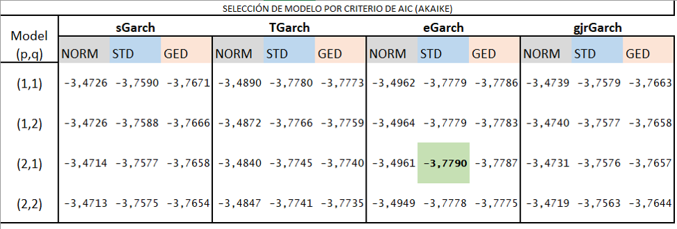
Se selecciona el modelo eGarch (2,1) según el criterio de selección de Akaike. Se contrastará con el Garch generalizado (1,1). Se revisarán parámetros y comportamiento de errores.
4. Preparación de datos
BTCSP <- read.csv("C:/Users/Personal/Desktop/BTCSP.csv", sep=";")
precio<-BTCSP
library(zoo)
precio.zoo=zoo(precio[,-1], order.by=as.Date(strptime(as.character(precio[,1]), "%d.%m.%Y")))
library(rmgarch)library(PerformanceAnalytics)
model<- window(precio.zoo [,"BTC.Close"], start="2014-01-01")
model<- na.approx(na.trim(CalculateReturns(model), side="both"))
spec = ugarchspec()
print(spec)##
## *---------------------------------*
## * GARCH Model Spec *
## *---------------------------------*
##
## Conditional Variance Dynamics
## ------------------------------------
## GARCH Model : sGARCH(1,1)
## Variance Targeting : FALSE
##
## Conditional Mean Dynamics
## ------------------------------------
## Mean Model : ARFIMA(1,0,1)
## Include Mean : TRUE
## GARCH-in-Mean : FALSE
##
## Conditional Distribution
## ------------------------------------
## Distribution : norm
## Includes Skew : FALSE
## Includes Shape : FALSE
## Includes Lambda : FALSE##
## *---------------------------------*
## * GARCH Model Fit *
## *---------------------------------*
##
## Conditional Variance Dynamics
## -----------------------------------
## GARCH Model : sGARCH(1,1)
## Mean Model : ARFIMA(1,0,1)
## Distribution : norm
##
## Optimal Parameters
## ------------------------------------
## Estimate Std. Error t value Pr(>|t|)
## mu 0.002540 0.001101 2.3077 0.021014
## ar1 0.814833 0.382341 2.1312 0.033075
## ma1 -0.791863 0.402468 -1.9675 0.049124
## omega 0.000125 0.000026 4.7669 0.000002
## alpha1 0.122571 0.020129 6.0893 0.000000
## beta1 0.825323 0.024812 33.2629 0.000000
##
## Robust Standard Errors:
## Estimate Std. Error t value Pr(>|t|)
## mu 0.002540 0.001164 2.1824 0.029081
## ar1 0.814833 0.541378 1.5051 0.132296
## ma1 -0.791863 0.565336 -1.4007 0.161305
## omega 0.000125 0.000074 1.6862 0.091765
## alpha1 0.122571 0.033899 3.6158 0.000299
## beta1 0.825323 0.052460 15.7325 0.000000
##
## LogLikelihood : 2788.191
##
## Information Criteria
## ------------------------------------
##
## Akaike -3.4712
## Bayes -3.4511
## Shibata -3.4713
## Hannan-Quinn -3.4638
##
## Weighted Ljung-Box Test on Standardized Residuals
## ------------------------------------
## statistic p-value
## Lag[1] 0.1034 0.7478
## Lag[2*(p+q)+(p+q)-1][5] 1.3352 0.9995
## Lag[4*(p+q)+(p+q)-1][9] 4.7756 0.5055
## d.o.f=2
## H0 : No serial correlation
##
## Weighted Ljung-Box Test on Standardized Squared Residuals
## ------------------------------------
## statistic p-value
## Lag[1] 0.3453 0.5568
## Lag[2*(p+q)+(p+q)-1][5] 1.0215 0.8548
## Lag[4*(p+q)+(p+q)-1][9] 1.3170 0.9692
## d.o.f=2
##
## Weighted ARCH LM Tests
## ------------------------------------
## Statistic Shape Scale P-Value
## ARCH Lag[3] 0.2712 0.500 2.000 0.6025
## ARCH Lag[5] 0.3865 1.440 1.667 0.9165
## ARCH Lag[7] 0.4865 2.315 1.543 0.9796
##
## Nyblom stability test
## ------------------------------------
## Joint Statistic: 1.3331
## Individual Statistics:
## mu 0.32344
## ar1 0.03306
## ma1 0.03301
## omega 0.10592
## alpha1 0.07153
## beta1 0.10984
##
## Asymptotic Critical Values (10% 5% 1%)
## Joint Statistic: 1.49 1.68 2.12
## Individual Statistic: 0.35 0.47 0.75
##
## Sign Bias Test
## ------------------------------------
## t-value prob sig
## Sign Bias 1.0648 0.2871
## Negative Sign Bias 1.1088 0.2677
## Positive Sign Bias 0.7929 0.4279
## Joint Effect 1.9171 0.5898
##
##
## Adjusted Pearson Goodness-of-Fit Test:
## ------------------------------------
## group statistic p-value(g-1)
## 1 20 286.9 9.624e-50
## 2 30 299.4 1.056e-46
## 3 40 316.5 3.768e-45
## 4 50 329.7 3.034e-43
##
##
## Elapsed time : 5.006171garch112e2.2.2.spec = ugarchspec(mean.model = list(armaOrder = c(0,0)),
variance.model = list(garchOrder = c(2,1),
model = "eGARCH"), distribution.model = "std")
garch.fit112e2.2.2= ugarchfit(garch112e2.2.2.spec, data = model, fit.control=list(scale=TRUE))
print(garch.fit112e2.2.2)##
## *---------------------------------*
## * GARCH Model Fit *
## *---------------------------------*
##
## Conditional Variance Dynamics
## -----------------------------------
## GARCH Model : eGARCH(2,1)
## Mean Model : ARFIMA(0,0,0)
## Distribution : std
##
## Optimal Parameters
## ------------------------------------
## Estimate Std. Error t value Pr(>|t|)
## mu 0.001261 0.000528 2.3895 0.016871
## omega -0.098617 0.052158 -1.8908 0.058657
## alpha1 -0.091854 0.062178 -1.4773 0.139602
## alpha2 0.112060 0.062577 1.7908 0.073330
## beta1 0.983072 0.008942 109.9359 0.000000
## gamma1 0.451433 0.099049 4.5577 0.000005
## gamma2 -0.137387 0.080693 -1.7026 0.088644
## shape 2.550534 0.186797 13.6540 0.000000
##
## Robust Standard Errors:
## Estimate Std. Error t value Pr(>|t|)
## mu 0.001261 0.000509 2.4788 0.013183
## omega -0.098617 0.070233 -1.4041 0.160275
## alpha1 -0.091854 0.065685 -1.3984 0.161993
## alpha2 0.112060 0.064881 1.7272 0.084139
## beta1 0.983072 0.012533 78.4368 0.000000
## gamma1 0.451433 0.107693 4.1918 0.000028
## gamma2 -0.137387 0.085209 -1.6124 0.106885
## shape 2.550534 0.197290 12.9278 0.000000
##
## LogLikelihood : 3036.887
##
## Information Criteria
## ------------------------------------
##
## Akaike -3.7790
## Bayes -3.7522
## Shibata -3.7791
## Hannan-Quinn -3.7691
##
## Weighted Ljung-Box Test on Standardized Residuals
## ------------------------------------
## statistic p-value
## Lag[1] 3.322 0.06836
## Lag[2*(p+q)+(p+q)-1][2] 4.493 0.05561
## Lag[4*(p+q)+(p+q)-1][5] 7.590 0.03721
## d.o.f=0
## H0 : No serial correlation
##
## Weighted Ljung-Box Test on Standardized Squared Residuals
## ------------------------------------
## statistic p-value
## Lag[1] 0.1405 0.7078
## Lag[2*(p+q)+(p+q)-1][8] 0.7473 0.9883
## Lag[4*(p+q)+(p+q)-1][14] 1.9573 0.9920
## d.o.f=3
##
## Weighted ARCH LM Tests
## ------------------------------------
## Statistic Shape Scale P-Value
## ARCH Lag[4] 0.01235 0.500 2.000 0.9115
## ARCH Lag[6] 0.38116 1.461 1.711 0.9244
## ARCH Lag[8] 0.58042 2.368 1.583 0.9750
##
## Nyblom stability test
## ------------------------------------
## Joint Statistic: 2.4443
## Individual Statistics:
## mu 0.51929
## omega 0.17655
## alpha1 0.40823
## alpha2 0.42594
## beta1 0.14497
## gamma1 0.09465
## gamma2 0.09181
## shape 0.13315
##
## Asymptotic Critical Values (10% 5% 1%)
## Joint Statistic: 1.89 2.11 2.59
## Individual Statistic: 0.35 0.47 0.75
##
## Sign Bias Test
## ------------------------------------
## t-value prob sig
## Sign Bias 1.0846 0.2783
## Negative Sign Bias 0.4547 0.6494
## Positive Sign Bias 1.4585 0.1449
## Joint Effect 3.0063 0.3907
##
##
## Adjusted Pearson Goodness-of-Fit Test:
## ------------------------------------
## group statistic p-value(g-1)
## 1 20 38.41 0.005261
## 2 30 38.43 0.113098
## 3 40 53.32 0.062957
## 4 50 50.24 0.423920
##
##
## Elapsed time : 7.8885685. Revisión de parámetros del modelo eGarch (2,1)
 mu: Es el rendimiento promedio diario a “LARGO PLAZO.” Según el modelo, el BTC tenderá a un rendimiento diario del 0,1% en el largo plazo. Con un P-valor significativo menor a 5%.
omega: Es la varianza a largo plazo del retorno del BTC, en este
caso alrededor del 9% (volatilidad). P-valor no significativo 5.8%.
caso alrededor del 9% (volatilidad). P-valor no significativo 5.8%.
alpha 1: Es el impacto de la varianza cuadrada rezagada en el retorno de hoy. El rendimiento se explica un 9% por la volatilidad de hace un día. P-valor no significativo.
alpha 2: El rendimiento se explica en un 11 % por la volatilidad del 2 día anterior. P-valor no significativo.
beta 1: Es el impacto de los residuos cuadrados rezagados en el rendimiento y se explica un 98% por la varianza ajustada del día anterior. P-valor significativo.
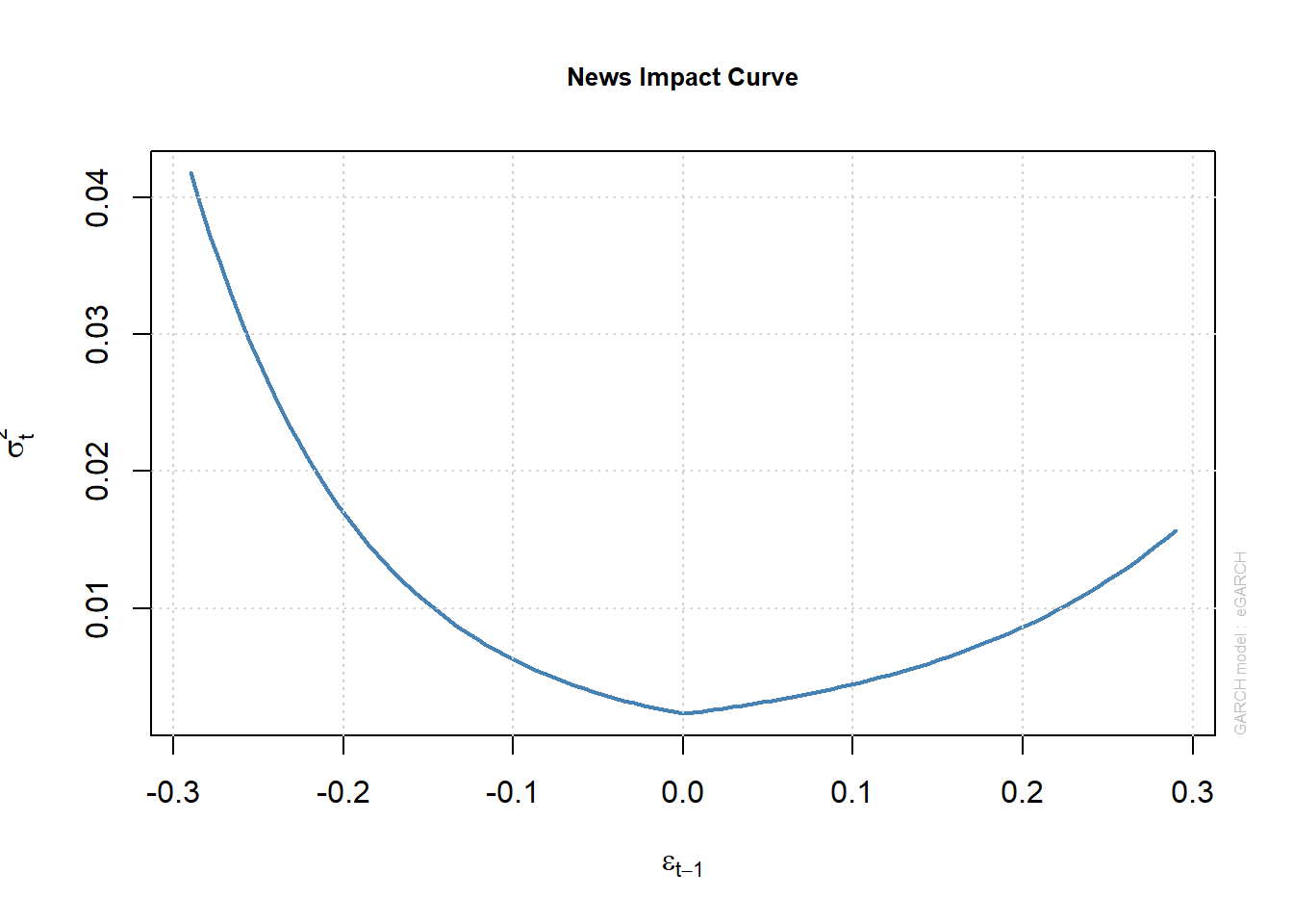
gamma 1: Son los parámetros de apalancamiento. El valor positivo indica que el los retornos del BTC tienen efecto de apalancamiento,
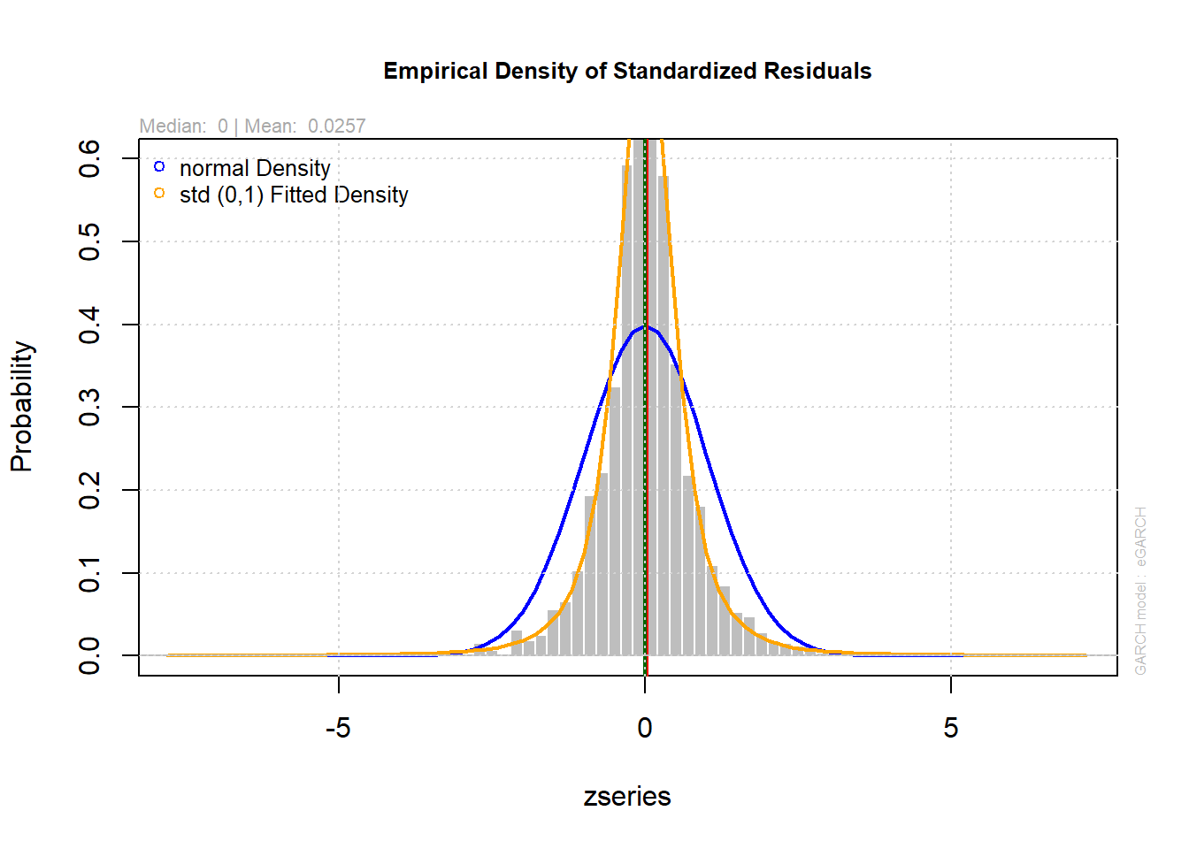
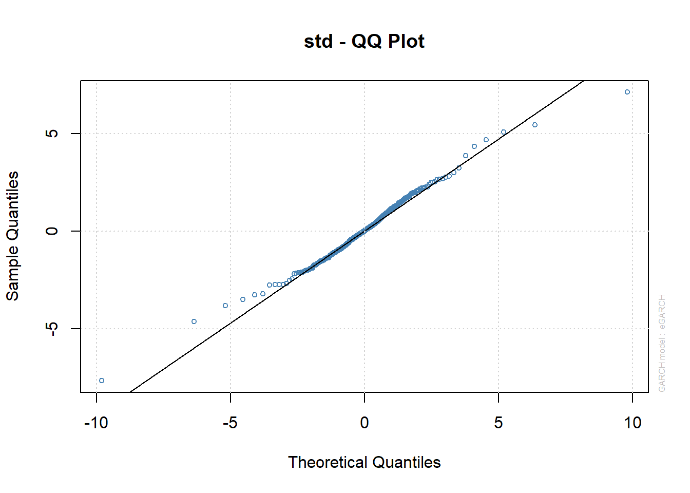
Shape: Son los grados de libertad de la distribución t de Student y cuanto más grande más gruesa es la cola.
Diagnóstico del modelo
Es esencial realizar una verificación de diagnóstico en el modelo después de determinar el mejor modelo y su distribución correspondiente para el término de error para establecer si el modelo y la distribución están especificados correctamente. Este ejercicio emplea las pruebas Ljung-Box y Multiplicador de Lagrange (LM) para evaluar la presencia de autocorrelación y efectos ARCH respectivamente. La presencia de autocorrelación y efectos ARCH para los residuos tanto del modelo medio como de los modelos de volatilidad se probará utilizando estos dos diagnósticos.
6. Ljung Box
La prueba de Ljung Box se usa para probar si existen autocorrelaciones en los residuos de un modelo. La hipótesis nula de la prueba de Ljung-Box no se rechaza al nivel de significancia del 5%. Esto indica que los residuos estandarizados se consideran ruido blanco.
7. Prueba efecto ARCH LM
La prueba ponderada ARCH LM indica que no hay efecto ARCH en los modelos. Estas pruebas sugieren que el modelo eGarch mejor ajustado es suficiente para corregir la correlación en serie de las series de retorno en la ecuación de varianza condicional.
garch.fit = ugarchfit(garch112e2.2.2.spec, data = model, fit.control=list(scale=TRUE))
plot(garch.fit, which=3)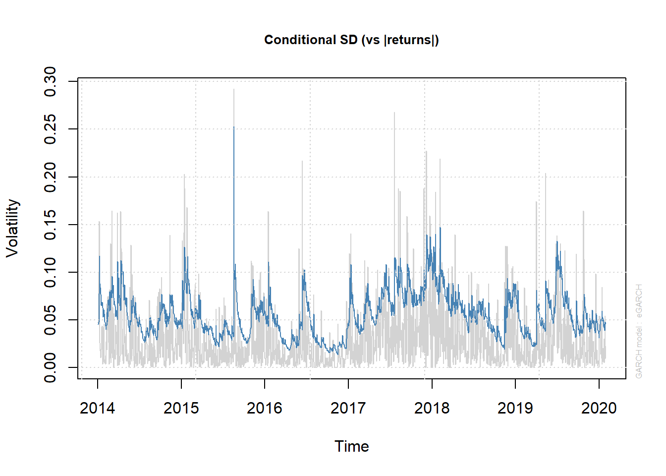
##
## please wait...calculating quantiles...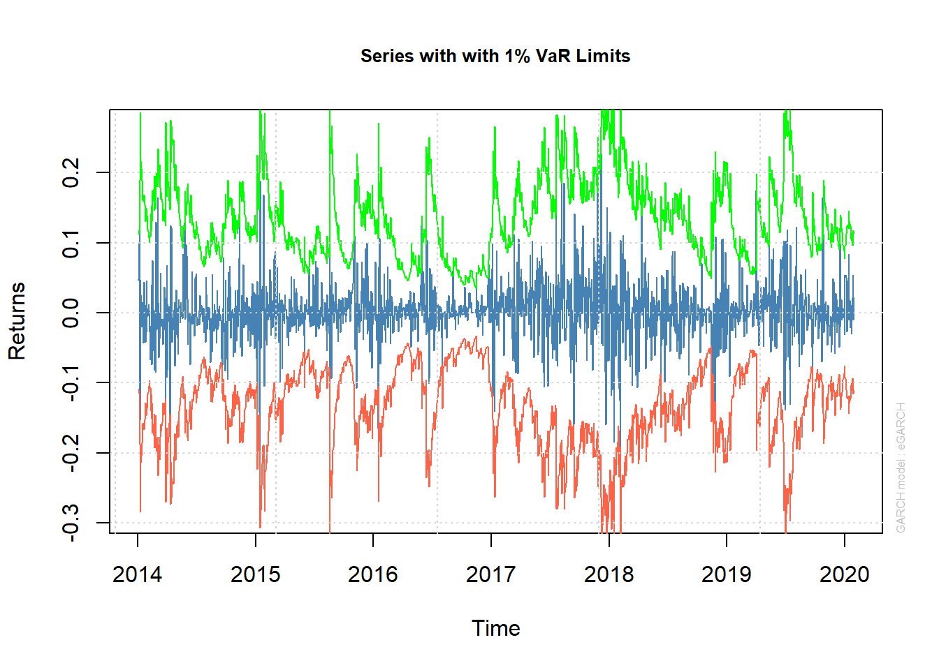
8. Valor en Riesgo VaR
Para validar el rendimiento del modelo eGARCH mejor ajustado, es útil realizar una prueba de respaldo histórica para comparar el Valor en riesgo estimado (VaR) con el rendimiento real durante el período de estudio. Si el retorno es menor que el VaR en la mayoría de los casos, tenemos un exceso de VaR. En este ejercicio, se establece una superación de VaR solo en el 1% de los casos, por lo tanto, las pruebas se evalúan en el nivel de significancia del 1%. El período de inicio de la prueba retrospectiva se establece 500 días después del comienzo de la serie (finales 2015). Además, los parámetros eGARCH se actualizan posteriormente en todo el conjunto de datos utilizando la estimación de la ventana móvil en lugar de mantenerse constante en el tiempo. Esto se hace para lograr flexibilidad en los parámetros.
Retornos del Bitcoins con límites del VaR al 1%
Las estimaciones del VaR producidas por el modelo de volatilidad son evaluadas por la prueba de cobertura incondicional de Kupiec y la prueba de independencia de Christoffersen.
Las pruebas se evalúan en el nivel de significancia del 1%, por lo tanto, se rechaza la hipótesis nula y el modelo se descarta posteriormente, si el valor p está por debajo del uno por ciento.
Los retornos de los datos alcanzan el 1% Var (Rojo) 9 veces en comparación con las 11 veces esperadas, no se rechaza la hipótesis nula de que las superaciones son correctas e independientes. Esto implica que se espera que una pérdida del 0,8% se supere solo el 1% del tiempo.
En el modelo se ha sobreestimado el riesgo de perder dinero.
Cobertura VaR y validación del modelo Interpretación de la cobertura VaR con probabilidad de pérdida α (1%):
El modelo de predicción válido tiene una cobertura cercana al nivel de probabilidad α usado:
- Si la cobertura ≫ α: tiene demasiadas superaciones: el cuantil pronosticado debería ser más negativo. En este caso se ha subestimado el riesgo de perder dinero.
- Si la cobertura ≪ α: tiene muy pocas superaciones, el cuantil pronosticado también fue negativo. En este caso se ha sobreestimado el riesgo de perder dinero.
garchroll <- ugarchroll(garch112e2.2.2.spec, data = model, n.start =500,
                        refit.window = "moving"
                        , refit.every = 100)
garchVaR <- quantile(garchroll, probs=0.01)
actual <- xts(as.data.frame(garchroll)$Realized, time(garchVaR))

mean(actual < garchVaR)
## [1] 0.008159565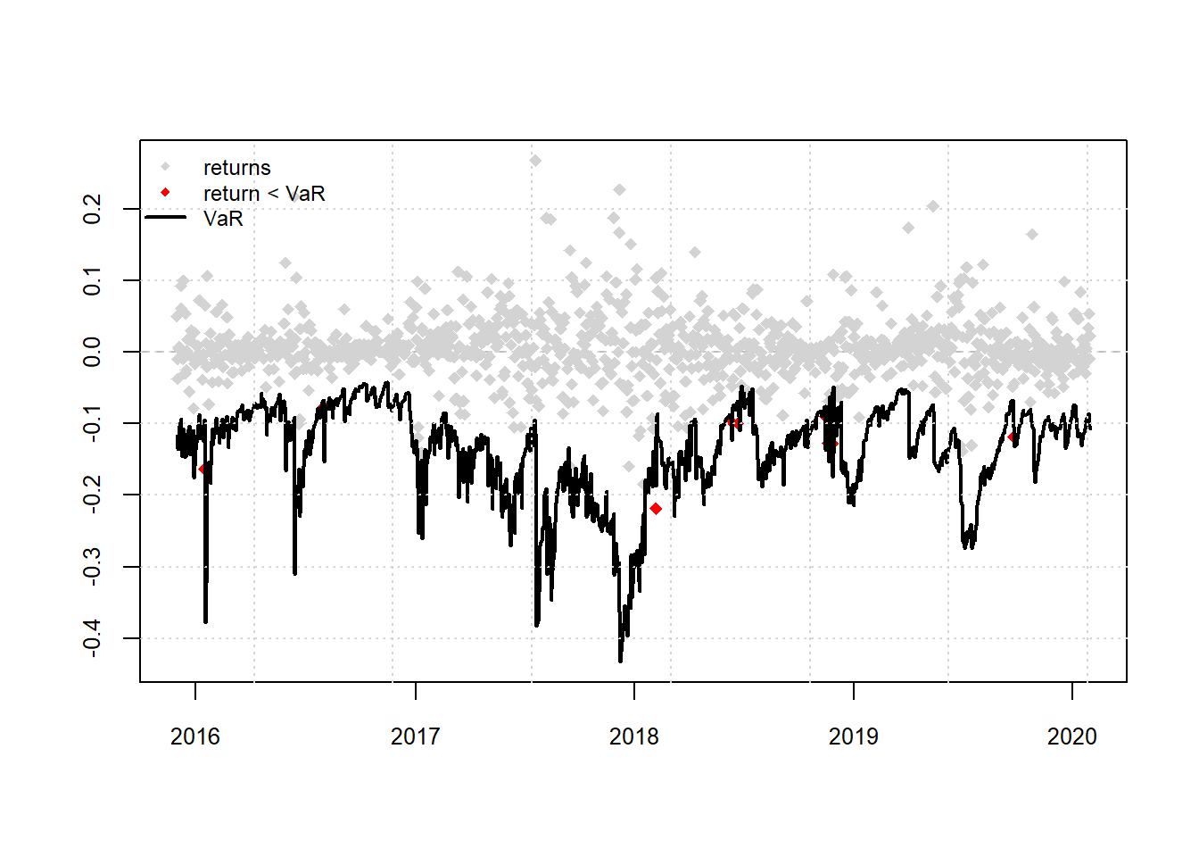
## VaR Backtest Report
## ===========================================
## Model:               eGARCH-std
## Backtest Length: 1103
## Data:
##
## ==========================================
## alpha:               1%
## Expected Exceed: 11
## Actual VaR Exceed:   9
## Actual %:            0.8%
##
## Unconditional Coverage (Kupiec)
## Null-Hypothesis: Correct Exceedances
## LR.uc Statistic: 0.403
## LR.uc Critical:      6.635
## LR.uc p-value:       0.526
## Reject Null:     NO
##
## Conditional Coverage (Christoffersen)
## Null-Hypothesis: Correct Exceedances and
##                  Independence of Failures
## LR.cc Statistic: 0.551
## LR.cc Critical:      9.21
## LR.cc p-value:       0.759
## Reject Null:     NO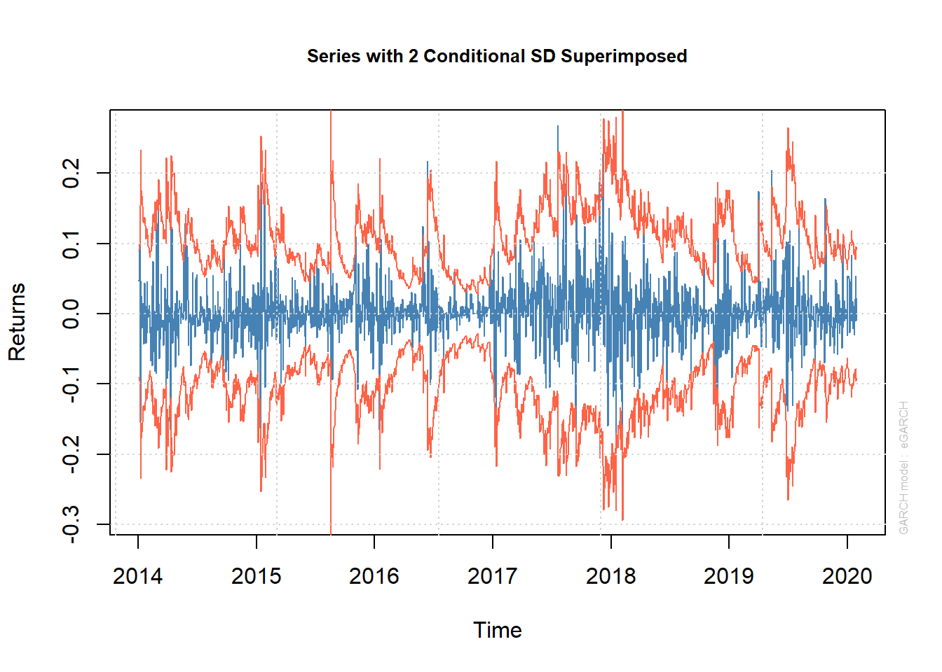
9. Análisis de residuos
##
## please wait...calculating quantiles...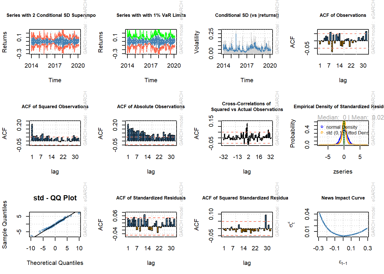
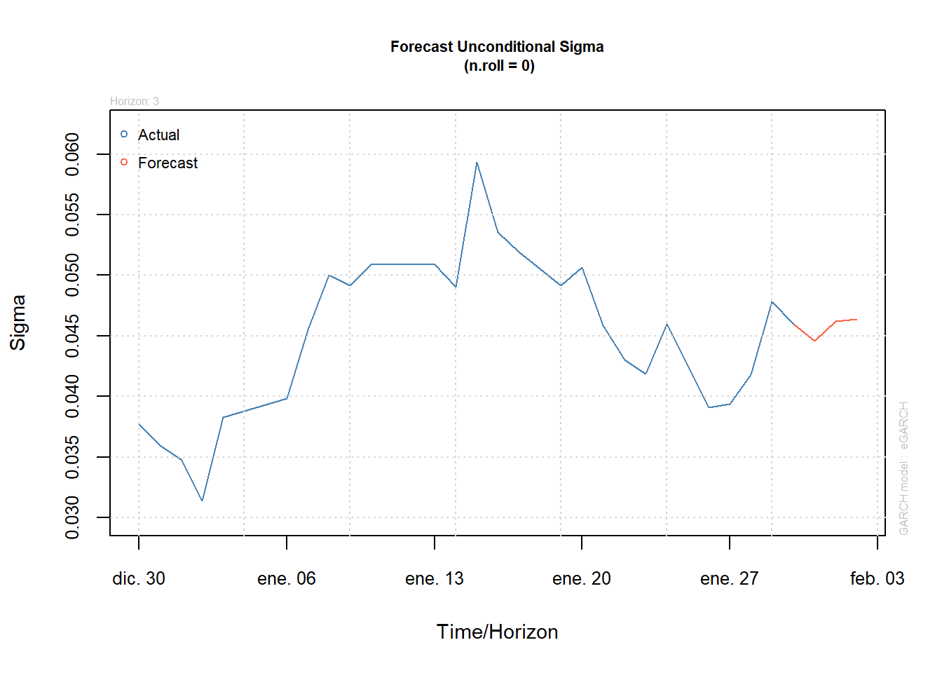
10. Pronósticos
1er Método
El comando n.ahead indica cuántos períodos se requieren pronosticar. Si es más de 1 período, los datos anteriores ya no son suficientes y el método utiliza el valor de pronóstico del pronóstico; da un paso adelante para calcular el pronóstico de dos períodos. Los pronósticos para la volatilidad están dados por sigma y el 1% de VaR se aplica a cada período. Ejem: Para el período T+1 la volatilidad esperada es 0.001261 y el VaR del 1% es 0.04461.
##
## *------------------------------------*
## *       GARCH Model Forecast         *
## *------------------------------------*
## Model: eGARCH
## Horizon: 3
## Roll Steps: 0
## Out of Sample: 0
##
## 0-roll forecast [T0=2020-01-30]:
##       Series   Sigma
## T+1 0.001261 0.04461
## T+2 0.001261 0.04622
## T+3 0.001261 0.04635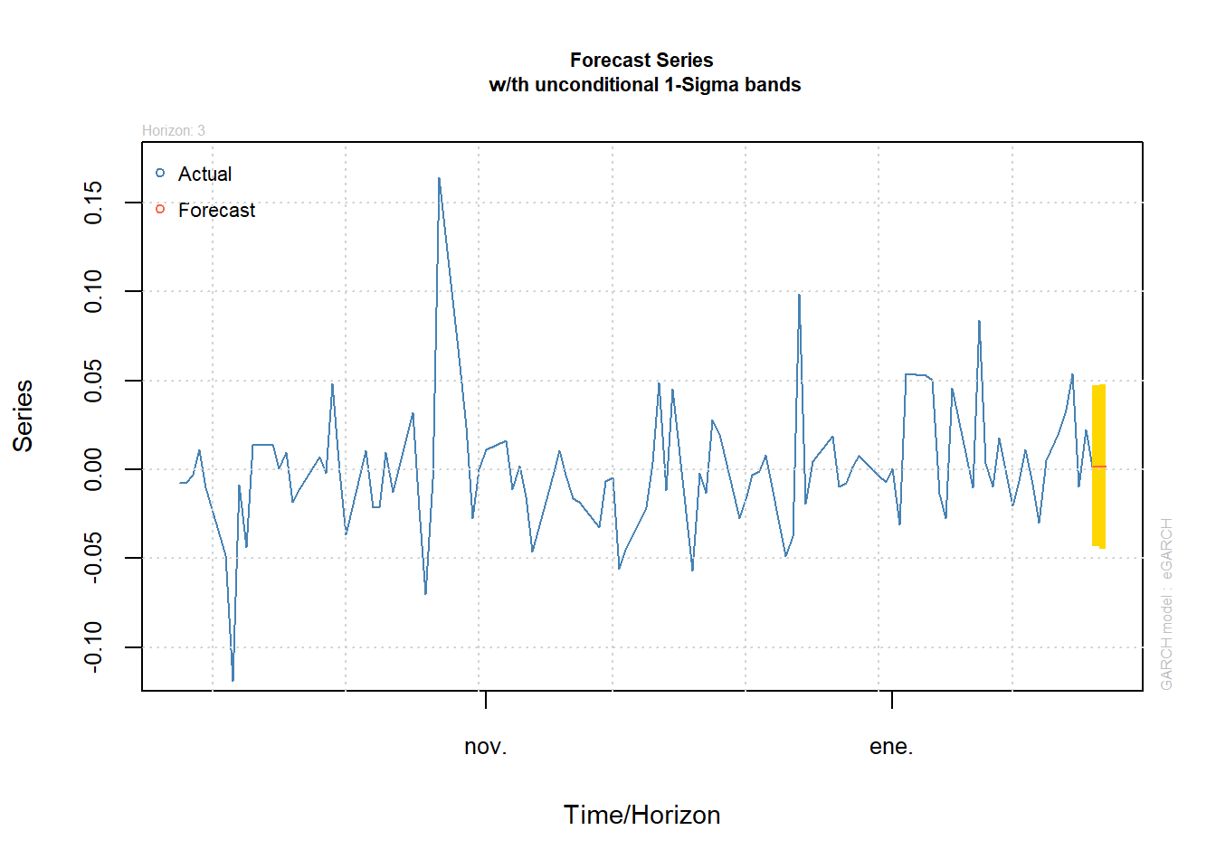
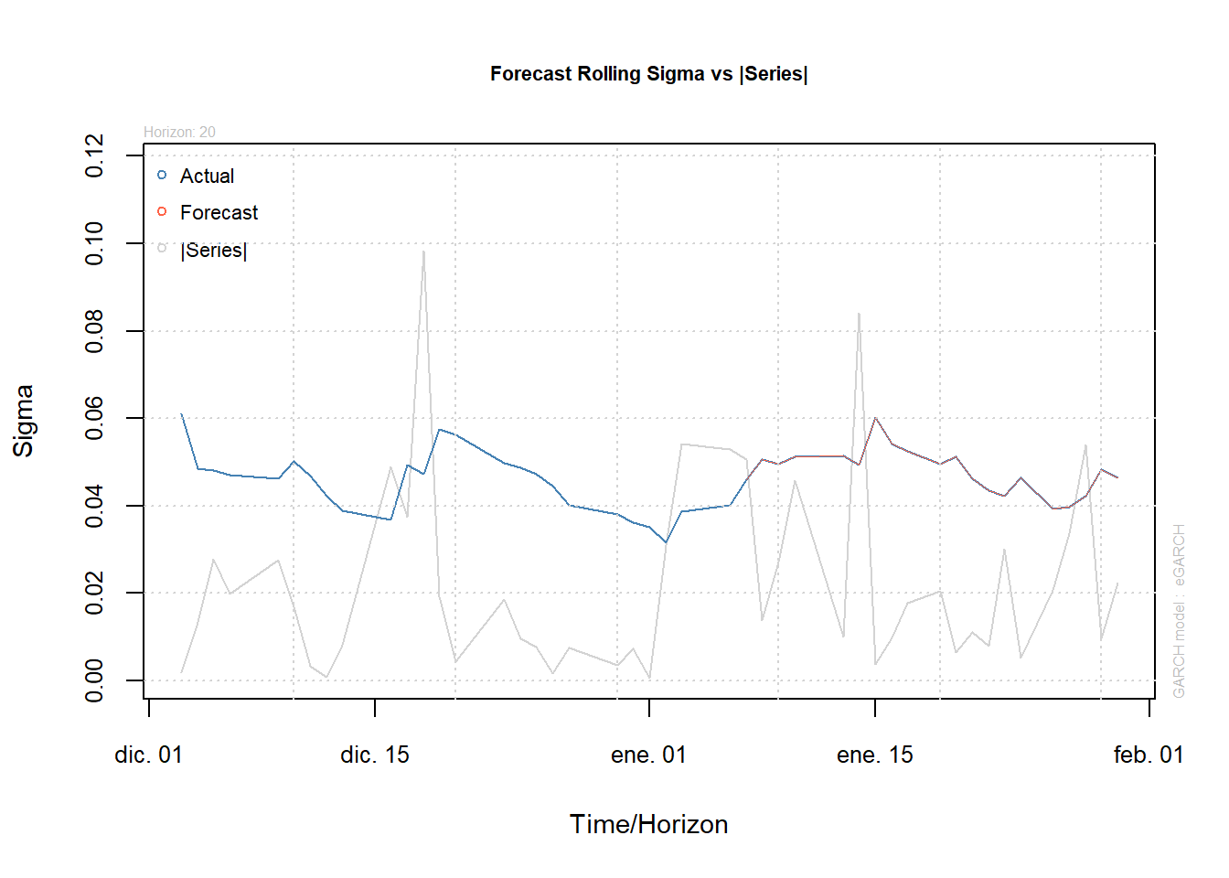
2do Método
Con el método forecast rolling se pueden hacer pronósticos manipulando los períodos de la serie dentro del histórico y seleccionando los datos que se dejan por fuera y así tener otro método de pronósticos. Forecast rolling n.roll nos da el número de pronósticos n-ahead. Entonces, desliza la ventana sobre el histórico y hace el siguiente pronóstico n-ahead. Out.sample se usa para definir las observaciones que deben excluirse en el procedimiento de estimación para realizar pronósticos fuera de la muestra.
modelfit=ugarchfit(garch112e2.2.2.spec,data=model, solver="hybrid", out.sample=20)
modelforecast<-ugarchforecast(modelfit, data = NULL, n.ahead = 30, n.roll = 20, external.forecasts = list(mregfor = NULL, vregfor = NULL))
modelforecast
##
## *------------------------------------*
## * GARCH Model Forecast *
## *------------------------------------*
## Model: eGARCH
## Horizon: 30
## Roll Steps: 20
## Out of Sample: 20
##
## 0-roll forecast [T0=2020-01-06]:
## Series Sigma
## T+1 0.001214 0.04605
## T+2 0.001214 0.04710
## T+3 0.001214 0.04722
## T+4 0.001214 0.04734
## T+5 0.001214 0.04746
## T+6 0.001214 0.04758
## T+7 0.001214 0.04770
## T+8 0.001214 0.04781
## T+9 0.001214 0.04793
## T+10 0.001214 0.04804
## T+11 0.001214 0.04815
## T+12 0.001214 0.04826
## T+13 0.001214 0.04836
## T+14 0.001214 0.04847
## T+15 0.001214 0.04857
## T+16 0.001214 0.04867
## T+17 0.001214 0.04877
## T+18 0.001214 0.04887
## T+19 0.001214 0.04897
## T+20 0.001214 0.04907
## T+21 0.001214 0.04916
## T+22 0.001214 0.04926
## T+23 0.001214 0.04935
## T+24 0.001214 0.04944
## T+25 0.001214 0.04953
## T+26 0.001214 0.04962
## T+27 0.001214 0.04970
## T+28 0.001214 0.04979
## T+29 0.001214 0.04987
## T+30 0.001214 0.04995##
## GARCH Roll Mean Forecast Performance Measures
## ---------------------------------------------
## Model : eGARCH
## No.Refits : 12
## No.Forecasts: 1103
##
## Stats
## MSE 0.00209
## MAE 0.03024
## DAC 0.52400##
## GARCH Roll Mean Forecast Performance Measures
## ---------------------------------------------
## Model : sGARCH
## No.Refits : 12
## No.Forecasts: 1103
##
## Stats
## MSE 0.002107
## MAE 0.030420
## DAC 0.520400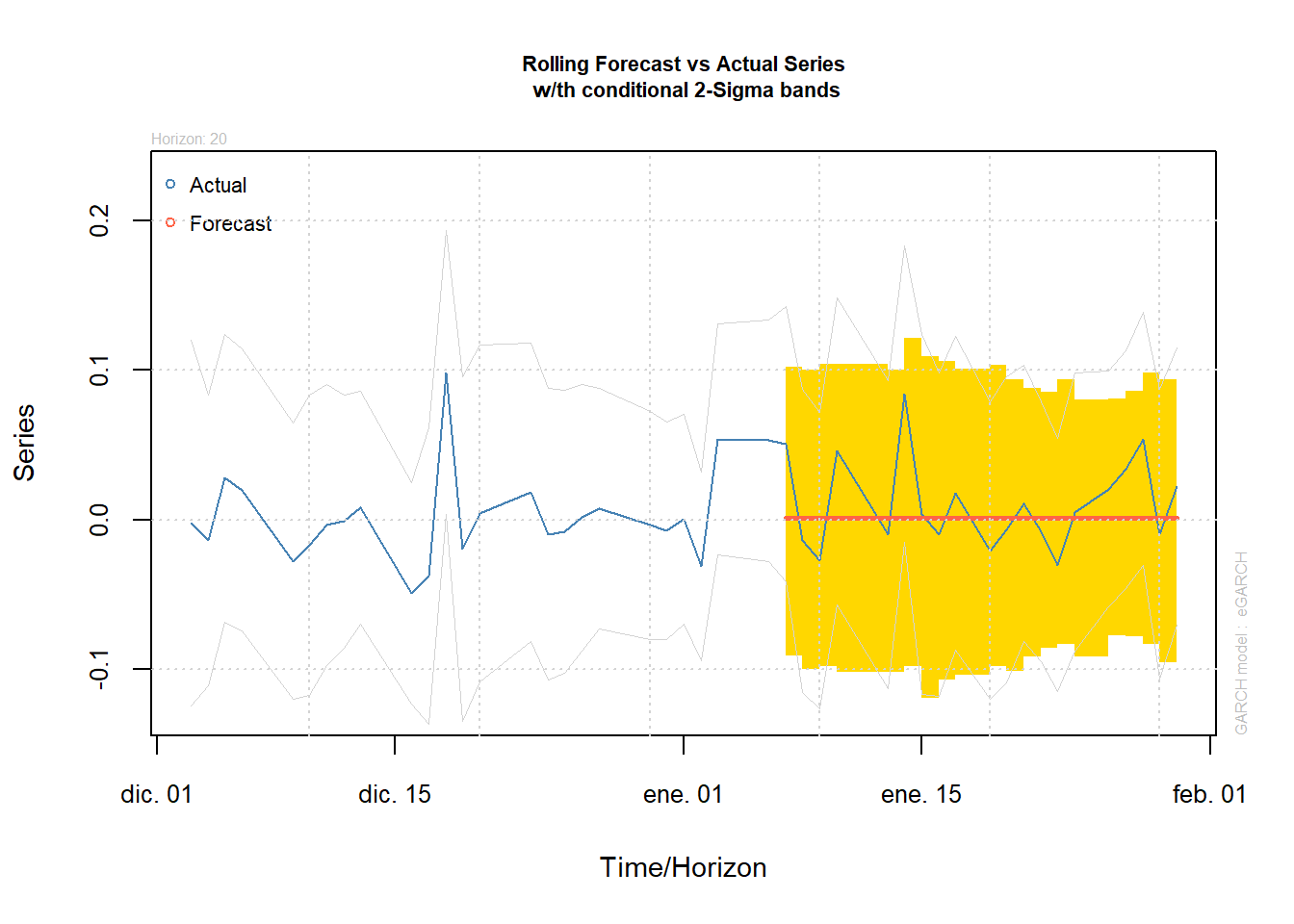
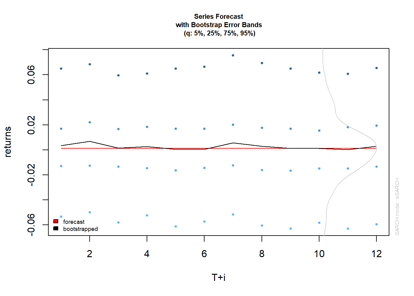
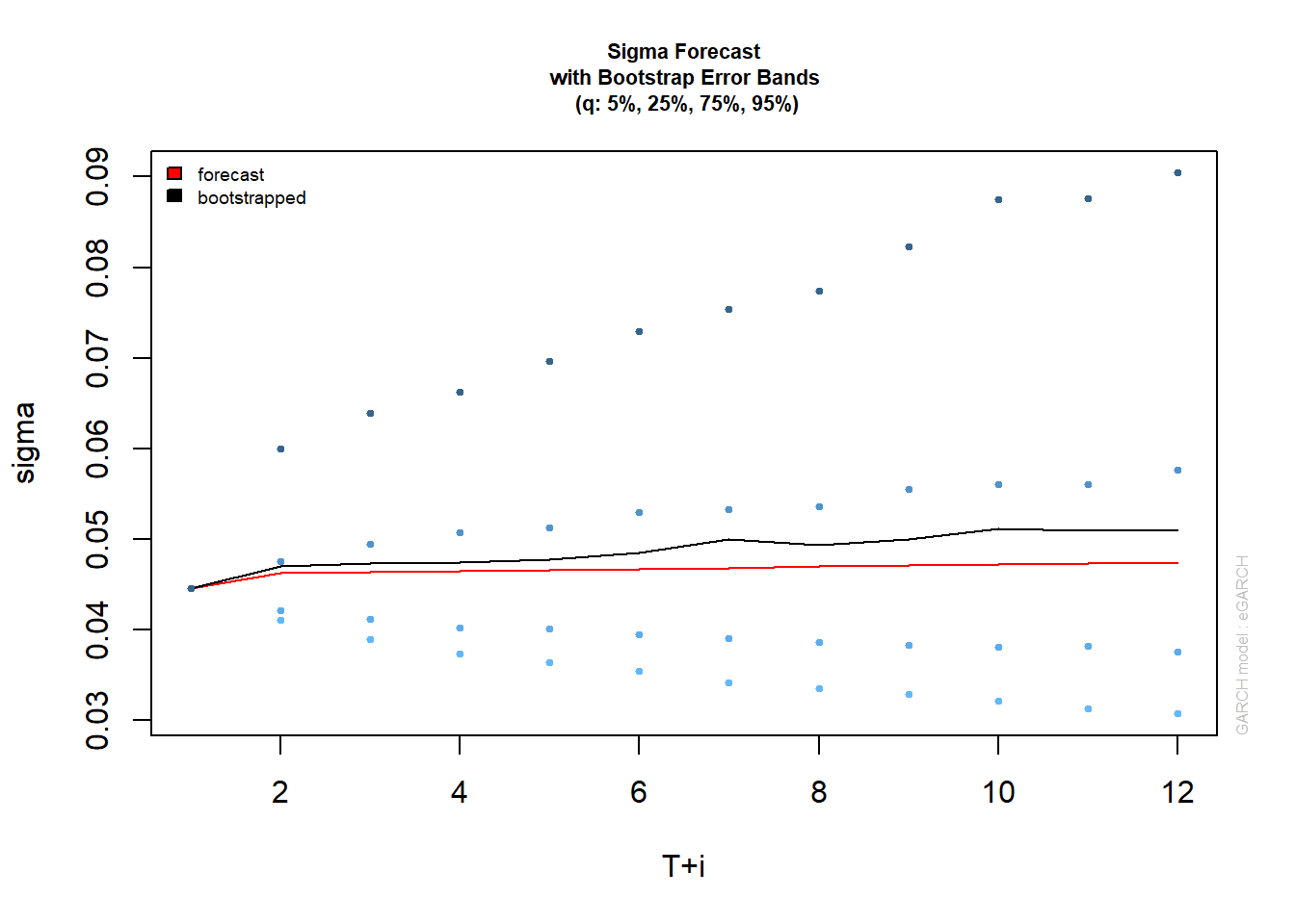
3er Método
Existen dos fuentes principales de incertidumbre sobre el pronóstico anticipado de los modelos Garch, el que surge de la forma de la densidad predictiva y el otro debido a la estimación de parámetros. El método bootstrap se basa en innovaciones de muestreo de la distribución empírica del modelo Garch ajustado para generar estimaciones futuras de la serie y del valor sigma. El método “parcial”, solo considera la incertidumbre de distribución y, aunque es más rápido, no generará intervalos de predicción para el pronóstico de sigma (1) para el cual solo la incertidumbre del parámetro es relevante en los modelos de tipo Garch.
bootp=ugarchboot(garch.fit,method=c("Partial","Full")[1],n.ahead = 12,n.bootpred=1000,n.bootfit=1000)
bootp
##
## *-----------------------------------*
## * GARCH Bootstrap Forecast *
## *-----------------------------------*
## Model : eGARCH
## n.ahead : 12
## Bootstrap method: partial
## Date (T[0]): 2020-01-30
##
## Series (summary):
## min q.25 mean q.75 max forecast[analytic]
## t+1 -0.34122 -0.012918 0.003356 0.017043 0.31886 0.001261
## t+2 -0.20763 -0.012533 0.006871 0.022018 0.34953 0.001261
## t+3 -0.20595 -0.013358 0.001464 0.016831 0.17488 0.001261
## t+4 -0.19842 -0.014634 0.002776 0.018565 0.31764 0.001261
## t+5 -0.20414 -0.016399 0.000498 0.016992 0.21584 0.001261
## t+6 -0.49729 -0.014409 0.000358 0.017074 0.27964 0.001261
## t+7 -0.29973 -0.012481 0.005515 0.020261 0.52718 0.001261
## t+8 -0.18334 -0.016198 0.002855 0.017824 0.30386 0.001261
## t+9 -0.36912 -0.016468 0.001129 0.016847 0.51179 0.001261
## t+10 -0.38256 -0.014856 0.001165 0.015573 0.33576 0.001261
## .....................
##
## Sigma (summary):
## min q0.25 mean q0.75 max forecast[analytic]
## t+1 0.044608 0.044608 0.044608 0.044608 0.044608 0.044608
## t+2 0.040791 0.042135 0.047028 0.047516 0.328326 0.046223
## t+3 0.037867 0.041156 0.047299 0.049411 0.159514 0.046350
## t+4 0.035179 0.040211 0.047443 0.050768 0.170167 0.046474
## t+5 0.032965 0.040053 0.047745 0.051209 0.156046 0.046597
## t+6 0.031812 0.039500 0.048474 0.053011 0.151017 0.046718
## t+7 0.029778 0.039090 0.049993 0.053324 0.473618 0.046838
## t+8 0.028666 0.038618 0.049374 0.053551 0.237884 0.046955
## t+9 0.027220 0.038243 0.050007 0.055505 0.197381 0.047071
## t+10 0.027007 0.038073 0.051173 0.056056 0.345446 0.047186
## .....................
Complementos:
Puedes compartir este material:
Referencias:
[2] Alejandro Vargas Sanchez (2017). Estimación de la Volatilidad de los Fondos de Inversión Abiertos en Bolivia. Centro de Investigación e Innovación en Finanzas (CIIFI). Recuperado de: http://www.scielo.org.bo/scielo.php?script=sci_arttext&pid=S2518-44312017000200003
Resultados de búsqueda
Resultado web con enlaces de partes del sit
Resultados de búsqueda
Resultado web con enlaces de partes del sitio
Por:
Jesús Benjamín Zerpa
Economista
JesusZerpaEconomia@Gmail.Com
 Excepto donde se indique lo contrario, el contenido de esta obra está bajo una licencia de Creative Commons Reconocimiento 4.0 Internacional.
| FINANCE | INTELLIGENCE BUSSINES | FORECASTING | TIME SERIES | FINANCIAL DASHBOARD | FINANCIAL BUDGET | SPATIAL ECONOMETRICS |
| FINANCE | INTELLIGENCE BUSSINES | FORECASTING | TIME SERIES | FINANCIAL DASHBOARD | FINANCIAL BUDGET | SPATIAL ECONOMETRICS |